How we do RTT estimation at Boundary.

On the Boundary blog I posted a tutorial on how we use the RTT measurement algorithm described in RFC 1323. Boundary has since been acquired, so the post has been reproduced here.

An article based on this work was invited to CACM and republished in ACM Queue.

Passively Monitoring Network Round-Trip Times

This post describes how Boundary uses a well-known TCP mechanism to calculate round-trip times (RTTs) between any two hosts by passively monitoring TCP traffic flows, i.e., without actively launching ICMP echo requests (pings). The post is primarily an overview of this one aspect of TCP monitoring, it also outlines the mechanism we are using, and demonstrates its correctness.

Introduction

Understanding network delay is key to understanding some important aspects of your network performance. The time taken to traverse the network between two hosts affects how responsive your services are, and can help you understand your service deployment or where your customers are located.

Boundary meters have been passively estimating round-trip times (RTT) between hosts by monitoring TCP flows for some time. The algorithm for calculating RTT from a TCP flow is documented in RFC 1323, and is commonly used by both end hosts on a connection to refine the timeout for retransmission of unacknowledged data when packets have been dropped or lost in the network. By calculating this value, hosts can optimise their network performance by having a better understanding of when loss may have occurred. Because it’s so useful, the mechanism is enabled by default in modern operating systems and is rarely blocked by firewalls, and thus appears in most TCP flows. (See the troubleshooting section of this post if is it not enabled for you.)

Boundary meters run the same algorithm on the traffic flows they monitor, and exports its RTT measurements for each flow once per second, and so we are able to provide an estimate of the RTTs that your TCP flows are actually experiencing. The RTT measure gathered by our meter will be close to the network RTT reported by ICMP. The two measures can differ in various ways: our measurement may be inflated if the TCP stack on one side delays an ACK, or if buffering in various places in the network incurs additional delay; equally, ICMP RTT may be higher if ICMP traffic is deprioritised in your network. In this post, my aim is to describe the basic RTT mechanism we’re using, and demonstrate its behaviour relative to ICMP pings.

In the first of the following three sections, I’ll outline how the algorithm operates, then describe my experimental setup that I used to generate the plots that follow.

RTT Calculation from TCP Flows

TCP offers a reliable byte stream to your applications, a significant part of which requires that TCP segments are retransmitted if they go missing between the source and destination (or, if an acknowledgement for a received segment goes missing between the destination and the source). In order to improve performance in all network conditions, the TCP stack requires round-trip time information to allow it to set its retransmission timeout (RTO) appropriately. TCP timestamps were defined to permit this calculation independently at both ends of a connection while data is being exchanged between the two hosts.

TCP timestamps are optional fields in the TCP header, so although they are extremely useful and usually present, they aren’t strictly required for TCP to function. The values are held in two 4-byte header fields: Timestamp Value (TSval) and Timestamp Echo Reply (TSecr). Both hosts involved in the connection emit TSval timestamps to the other host whenever a TCP segment is transmitted, and await the corresponding TSecr val in return. The time difference measured between first emitting a TSval and receiving it in a TSecr is the TCP stack’s best guess at a round-trip time. “Timestamp” here is an arbitrary value that increments at the granularity of the local system clock, and is not a timestamp that can be interpreted independently such as number of seconds since the epoch.

In the following diagram, time progresses top-to-bottom, and the grey lines indicate real time (let’s say in milliseconds) incrementing. Two hosts, A and B, have an open connection and are exchanging packets. In reality the two hosts have differing clocks, but for simplicity assume they are perfectly synchronised.

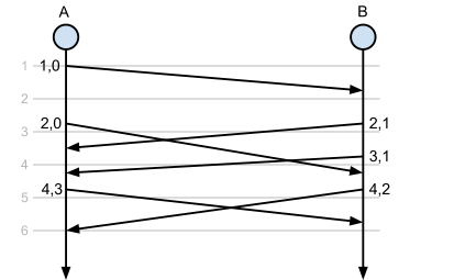
The example operates as follows:

• Host A emits a TCP segment which contains the timestamp options (TSval=1,TSecr=0), which host B receives at time 1; at time 2, B emits a TCP segment back to A which contains the values (TSval=2,TSecr=TSVal_A=1), which is received at A at time 3. Given this echoed value, A knows that the RTT in this instance is approximately 2ms.
• Similarly, the next segment that A emits carries TSval=4, and echoes the most recent timestamp from B, thus TSecr=TSVal_B=3. This is received by B at time 5, so B can calculate a similar RTT of 2ms.

Continuously sending values to the other host and noting the minimum time until the echo reply containing that value is received allows each end host to determine the RTT between it and the other host on a connection.

The caveat is that for a TSval to be useful, the TCP segment must be carrying data from the application. TCP segments can legitimately carry a zero-byte payload, most commonly when ACKing data. By requiring that the only valid TSvals come from TCP segments carrying data, the algorithm is less likely to measure breaks in the communication between the hosts. This implies that on a TCP flow in which data is exchanged exclusively in one direction, only one of the hosts will be able to calculate the RTT. Usually, however, there is some protocol chatter in both directions.

Finally, the meter attempts to make as few assumptions about its environment as possible. If the meter is running on a host which is routing traffic for other hosts, it will still estimate the RTT for the full flow between any two endpoints that its carrying traffic for; it will simply total the RTT calculated for both “sides” of the connection.

Monitoring Setup

Fundamentally, what we want to know is that Boundary’s RTT measurements match the “ground truth” of ICMP RTT measurements. To achieve this in a relatively controlled manner, I used the following configuration:

• I’m running two EC2 instances, both Ubuntu 12.04 LTS, one located in us-west-1c and one located in us-east-1a. By choosing hosts located so far apart, I have some natural latency on-path of approximately 80ms. The hosts are both configured with a bridge interface, br0, which only contains eth0; the purpose of this setup is to permit layer-2 control over network characteristics.
• Each host is running the current latest version of bprobe (v.1.0.0fi917). Both meters are talking locally to a dummy IPFIX collector we use internally that generates the output used to create the plots for this blog post.
• The Linux tool tc (Traffic Control) is used later to introduce additional path latency.
• All other network configuration, including parameters such as txqueuelen and TCP buffer sizes are maintained at their default settings.
• A bidirectional traffic flow is generated using iperf, for the meter to measure and calculate RTTs from.
• ICMP pings are measured simultaneously during each test.
• Each test runs for three minutes.

RTT Measurements

Given the setup described above, the first thing to do is set up an iperf flow and let the meters in both locations measure the output. In the following plots, orange and red represent ICMP RTTs, while blue and green represent TCP RTTs.

The first plot demonstrates the observed RTT calculated by the Boundary meter on both hosts during a three minute iperf trace, alongside the ICMP RTTs from both hosts. No additional latency was added at either end. The measurements look like the following:

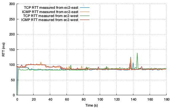
What’s pleasing here is that the meter strikes an RTT measurement that is remarkably close to the RTT measured by ICMP for the majority of the test. Measured from ec2-west, the median difference between ICMP and TCP RTT measured is 2.1ms; measured from ec2-east, the median difference measured is 0.2ms. That’s good news! Regardless, there are two regions to note:

1. During the first 40-50 seconds, ICMP traffic consistently estimates network RTTs marginally higher than the TCP flows suggest, probably an artifact of ICMP traffic deprioritisation given how stable the TCP measure is.
2. At around 135s, some network jitter is experienced, which is reported by both ICMP measures and is shown to manifest in both RTT measures. What’s likely is that the packets were buffered a little longer somewhere in the network but still arrived. The TCP metric is passive and relies on data being exchanged, and so sometimes can fall a little behind the active ICMP metric.

So let’s deliberately fool around with link latencies to make sure that the meter keeps up with what’s happening to the traffic if the network conditions change. For the next plot, I run precisely the same experiment as above, but intermittently increase the latency at each end (by 10ms on each side for all ingress and egress traffic, once every 18 seconds for the full three minute run). The resulting RTT measurements are as follows:

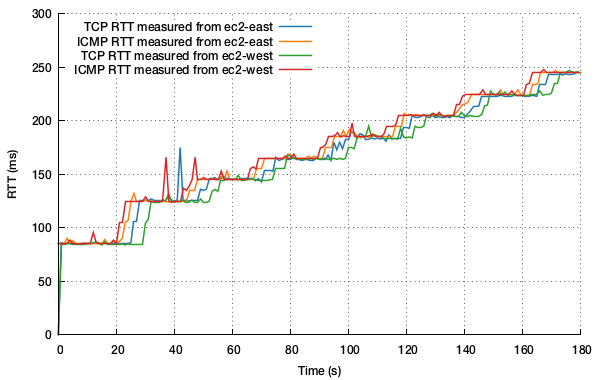
This plot is more interesting. Measured from ec2-west, the median difference between ICMP and TCP RTT measured is 2.8ms; measured from ec2-east, the median difference measured is 2.0ms. But what we also see is the ICMP ping measurement leading the meter’s RTT measurements by a second or two. So the meter can take a few moments longer to react to the change in network latency, but catches up as soon as TCP segments containing the appropriate TSval and TSecr values have been exchanged. Factors that are likely to prolong the response time to these changes are the time taken for TCP queues to drain at either side of a link, or TCP ACKing behaviour. Given the passive nature of this measurement, the meter does a pretty good job of keeping up.

What’s interesting, and reassuring, is just how close to the network RTT the meter actually gets every time in these experiments, without having to actively test your network at all.

In Conclusion

Calculating RTT is just one part of what Boundary aims to reveal about your network to help you understand what’s going on down there. This post has described how the basic RTT algorithm operates; in future posts, I hope to describe and demonstrate other TCP metrics and how network characteristics affect those. Some of the interactions between the factors that determine the health of your network can be non-trivial or unintuitive, and I hope to tease apart some of these for you.

Addendum: Troubleshooting

TCP timestamps are enabled by default on modern operating systems and by now are carried across most of the public Internet.

If you are using linux, you can check that you have TCP timestamps enabled by running:

cat /proc/sys/net/ipv4/tcp_timestamps

The output will be ‘1’ if timestamps are enabled; ‘0’ otherwise. To enable them, run (with appropriate privileges):

echo 1 > /proc/sys/net/ipv4/tcp_timestamps

All other major operating systems have similar configurations to enable these options.